2005年05月27日
gnuplot(5)
データファイルを使った3次元プロットについて。

# sin_cos_data.plt

set xrange [-3:3]; set yrange [-3:3]; set zrange [-2:2]
set xlabel "x"; set ylabel "y"; set zlabel "z"
set parametric
set hidden3d
splot "sin_cos.dat" with lines
# sin_cos.dat
#       x         y        z
-3.000000 -3.000000 0.139708
-3.000000 -2.900000 0.137022
-3.000000 -2.800000 0.132966
-3.000000 -2.700000 0.127583
-3.000000 -2.600000 0.120924
-3.000000 -2.500000 0.113057
-3.000000 -2.400000 0.104061
-3.000000 -2.300000 0.094025
-3.000000 -2.200000 0.083049
:
(省略)
sin_cos_data.c
#include <stdio.h>
#include <stdlib.h>
#include <string.h>
#include <math.h>

#define M_RANGE     3

int main(int argc, char *argv[])
{
    FILE    *fp;
    double  x, y, z;

    fp = fopen( "sin_cos.dat", "w" );

    for( x = -M_RANGE; x <= M_RANGE; x += 0.1 )
    {
        for( y = -M_RANGE; y <= M_RANGE; y += 0.1)
        {
            z = sin( x ) * cos( y );
            fprintf( fp, "%lf %lf %lf\n", x, y, z );
        }
        fprintf( fp, "\n" );
    }

    fclose(fp);

    return EXIT_SUCCESS;
}
今回は新しいコマンドとして set parametric と set hidden3d があります。
parametric モードは1行に x, y, z の3つの値を持つデータをプロットするモードです。また、ここでは示していませんが noparametric モードは z 値のみを持つ3次元データをプロットするときに使います。
hidden3d は陰線除去を行ってくれるコマンドです。ただ、この設定を行うとグラフの回転表示が非常に遅くなります。どうやら gnuplot はすべてソフトウェアで書かれているようですね。動作環境に応じて OpenGL や Direct3D (非Windows環境では無いので流石にこれは無理だと思いますが)で表示してもらえるといいのですが…。検索してみるとあったりして。
2005年05月26日
gnuplot(4)
3次元のグラフ表示について。今までは plot コマンドを使ってきましたが、ここでは splot を使います。

# sin(x)*cos(y)

set xrange [-3:3]; set yrange [-3:3]; set zrange [-2:2]
set xlabel "x"; set ylabel "y"; set zlabel "z"
splot sin(x)*cos(y)
ここでは軸のラベルもつけています。ラベルをつけるには xlabel, ylabel, zlabel コマンドを使います。
2005年05月25日
gnuplot(3)
さて、今度はテイラー展開です。
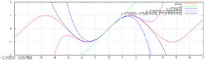
# taylar_sin.plt

set xrange [-7:7]; set yrange [-2:2]
plot sin(x)
replot x
replot x -x**3/(3*2)
replot x -x**3/(3*2) +x**5/(5*4*3*2)
replot x -x**3/(3*2) +x**5/(5*4*3*2) -x**7/(7*6*5*4*3*2)
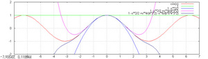
# taylar_cos.plt

set xrange [-7:7]; set yrange [-2:2]
plot cos(x)
replot 1
replot 1 -x**2/2
replot 1 -x**2/2 +x**4/(4*3*2)
replot 1 -x**2/2 +x**4/(4*3*2) -x**6/(6*5*4*3*2)
これらの展開に関しては様々な数学の専門書に書かれていると思いますが、一点あげるならオイラーの贈物をお薦めします。
2005年05月24日
gnuplot(2)
昨日に引き続き gnuplot でフーリエ級数です。
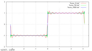
このグラフを表示するためのファイルはこれです。
# fourier_10-10000.plt

set xrange [-3.5:3.5]; set yrange [-2:2]
plot "fourier_10.dat" with line
replot "fourier_100.dat" with line
replot "fourier_10000.dat" with line
ここで使用されているファイルは以下にあります。グリッド表示には grid.plt を使います。
これらのデータファイルはpreformatエントリーで示したもので作成されています。というわけでxの範囲は-πからπまでとなります(このフォント、piがすごいですね)。
2005年05月22日
gnuplot(1)
試しにフーリエ級数を表示してみます。

このグラフを表示するためのファイルはこれです。
# fourier.plt

set xrange [-3.5:3.5]; set yrange [-2:2]
plot 4*sin(x)/pi +4*sin(3*x)/(3*pi) +4*sin(5*x)/(5*pi) +4*sin(7*x)/(7*pi) \
 +4*sin(9*x)/(9*pi)
replot 4*sin(x)/pi +4*sin(3*x)/(3*pi) +4*sin(5*x)/(5*pi) +4*sin(7*x)/(7*pi) \
 +4*sin(9*x)/(9*pi) +4*sin(11*x)/(11*pi)
replot 4*sin(x)/pi +4*sin(3*x)/(3*pi) +4*sin(5*x)/(5*pi) +4*sin(7*x)/(7*pi) \
 +4*sin(9*x)/(9*pi) +4*sin(11*x)/(11*pi) +4*sin(13*x)/(13*pi)
# grid.plt

set xtics 1
set ytics 1
set grid
replot
gnuplot ではいろいろな設定を行った後には replot コマンドを実行します。そうしないと設定が反映されません。
# なんかイマイチ movable type の使いこなしに難が。。
.pltファイルへのリンクを追加しました。
preformat
見え方のテスト。
#include <stdio.h>
#include <stdlib.h>
#include <string.h>
#include <math.h>

#define M_PI        3.141592

double term( int seriese, double x )
{
    return sin((2*seriese+1)*x) / (2*seriese+1);
}

int main(int argc, char *argv[])
{
    double  x, y;
    FILE    *fp;
    int     seriese, seriese_max;

    if( argc == 2 )
    {
        seriese_max = atoi(argv[1]);
        if( seriese_max == 0 )
            seriese_max = 10;
    }
    else
    {
        seriese_max = 10;
    }

    fp = fopen( "fourier.dat", "w" );

    for( x = -M_PI; x < M_PI; x += 0.001 )
    {
        y = 0;
        for( seriese = 0; seriese <= seriese_max; seriese++ )
        {
            y += term( seriese, x );
        }
        fprintf( fp, "%lf %lf\n", x, 4/M_PI*y );
    }

    fclose(fp);

    return EXIT_SUCCESS;
}
ここで終わり。
そろそろちゃんとgnuplotの覚書を書いていこう。。。
ん~、ソースコードを載せると行が凄いことになるなぁ。かつ、「テキストフォーマット」の変換があると<pre>タグ内も変換されるようで結構考えてしまいます。行間も<pre>タグ内はちょっと変えた方が読みやすそう…。ということでline-height: 120%にしてみました。
